Picture by Hermes Rivera

Lazy evaluation - Weaving infinities

A Quick Recap

We have been following the white paper by John Hughes¹. And so far we've touched upon the below.

1. Why FP Matters - Part 1 🐘 : A brief introduction - How FP can help improve developer productivity and the motivation for popular languages to adapt functional aspects.
2. Why FP Matters - Part 1½ 💫: A bit of Haskell - A bit of Haskell to get used to the syntax and the syntactic sugar.
3. Why FP Matters - Part 2 🎈: Higher-order functions - Basics of higher-order functions, partial-application and currying.
4. Why FP Matters - Part 2½ 🍰 - Slicing complexity with Higher-order functions - How to develop powerful and reusable functions to process lists and trees to demonstrate the power of higher-order functions.
5. Why FP Matters - Part 3 🎩 - Lazy evaluation - Conjuring infinities - Use lazy evaluation and function composition to write module code to process infinite streams. I recommend that you first go through Part 3 at least since it is where we started with basic programs using lazy evaluation. This post builds on that.

What we will cover in this post?

We will walk down the lane, yet again chasing infinite sequences. Looking for answers. More precisely we will look at ways to perform Numerical Differentiation and Numerical Integration. We will generate a series of approximations, just as we did in the previous post. Each of our approximations will be better than the previous and we will terminate our search when we are satisfied with the margin of error.

What will be different? Our algorithms for finding approximations and eliminating will get more sophisticated. We will see some math. But most importantly, we will see how the programs still retain their modularity. All with the help of our new friends - selectors and generators - whom we met in the previous post.

🎐 Numerical Differentiation

Picture by Félix Prado

We should refresh our memory of how derivates work. Differentiation or derivates tell us the rate of change at a particular point in space. You can read more about it on Wikipedia.

For our example, let's restrict ourselves to two-dimensions. Suppose we draw a curve displaying the relation of the values obtained by applying a function f to the corresponding values of x and then choose a point (say Xn) on that curve. Then the rate of change of the values at that point would be the derivate of the function f at Xn.

Turns out that the rate of change of a curve at a particular point is the slope of the curve at that point. This seems like a computable value but to get the slope of the curve at a point means that we break the curve up at that point into an infinitesimally small part. That infinitesimally small piece will look like a part of a straight line, and we know how to get the slope of a line in 2D.

There is one problem though, computers don't do infinitesimally small well. What do we do? We start with an approximation and keep reducing the length of the curve under inspection our values don't seem to change much. It will be bounded by the limits of our computing system but in most cases, it will be an acceptable approximation.

Animation by Sam Ogden

Version 1: Simple Differentiation using Numerical Methods ⭐

Say we have a function repeat', that takes in a function f and a seed value a. repeat' will produce a series of values starting with

• the original value of a, let's call it a0 followed by
• the next value which is obtained by apply f on a0, then
• the next value obtained by applying f on a0 twice, then
• the next value obtained by applying f on a0 thrice, and so on ...

repeat' f a = a : repeat' f (f a)

repeat' f a0 will produce the below sequence

a0, (f a0), (f (f a0)), (f (f (f a0))), ...

Note that this is a non-terminating sequence. You shouldn't be worried about it since we have dealt with one such sequence in the earlier post.

Now, we define a function easydiff' which takes in a function f, a point on the X-axis x and a distance h. This function is a simple one, which calculates the slope of the line considering the two points (x1, y1) and (x2, y2), where

x1 = x, y1 = (f x), x2 = x + h, and y2 = (f (x + h))

easydiff' f x h =
  ((f (x+h)) - (f x)) / h

Using the built-in map function to transform elements in a list, and using a simple function - halve' we can define the differentiate' function as below.

halve' x = x / 2
differentiate' f x h0 =
  map (easydiff' f x) (repeat' halve' h0)

Borrowing, the within' function from the last post, we can simply compute the derivative of the function sin at x=2, as follows. Note, that we start with the value of h as 1.

within' eps $ differentiate' sin 2 1

Putting together all the pieces of our first version of the differentiating program.

repeat' f a = a : repeat' f (f a)
within' eps (a1:a2:rest)
  | abs (a1 - a2) < eps = a2
  | otherwise = within' eps (a2:rest)
easydiff' f x h =
  ((f (x+h)) - (f x)) / h
halve' x = x / 2
differentiate' f x h0 =
  map (easydiff' f x) (repeat' halve' h0)

This wasn't much different from our previous program to compute square roots using the Newton Raphson method. Almost the same, apart from the fact that we use map.

map takes in a function f, and a list of values, and produces a new list, which has elements corresponding to the original list. Only, that the elements in the new list have been transformed by applying the function f on them.

We defined our own map' function in Part 2½, but that was a bit greedy. We used the in-built function map here as it is lazy and it works the same way, except that it is lazy and it would transform the input elements as they pass through it. We can easily implement a lazy map ourselves, you can try it out on your own.

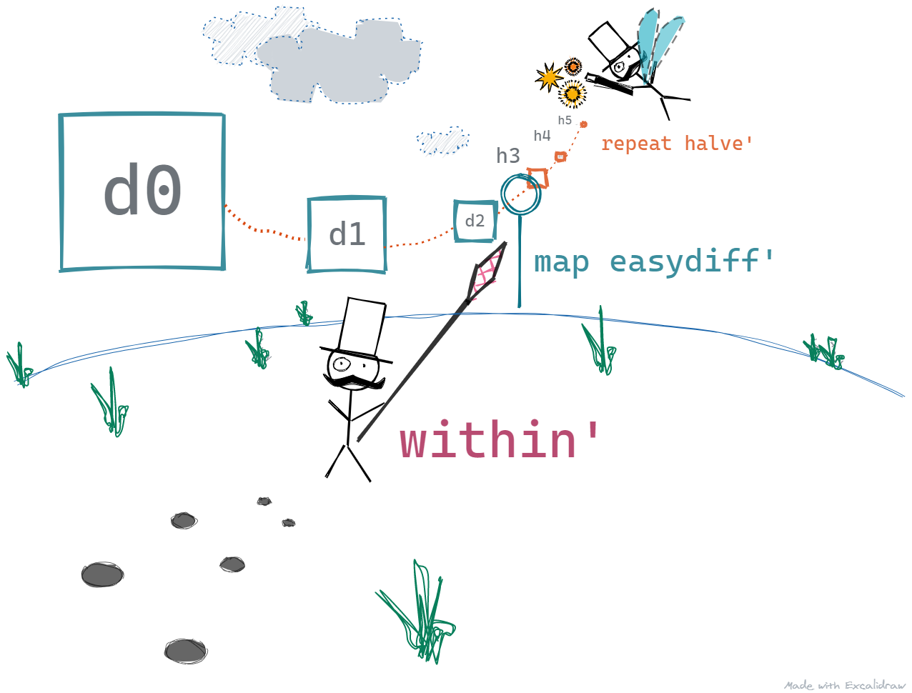
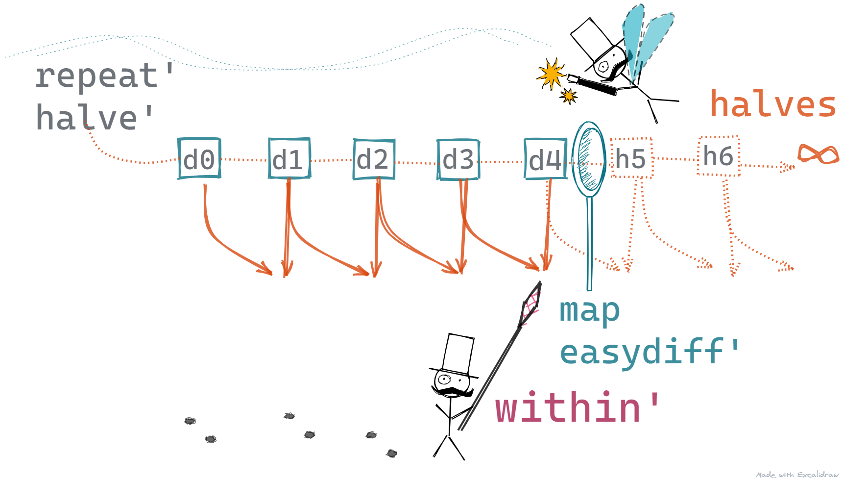
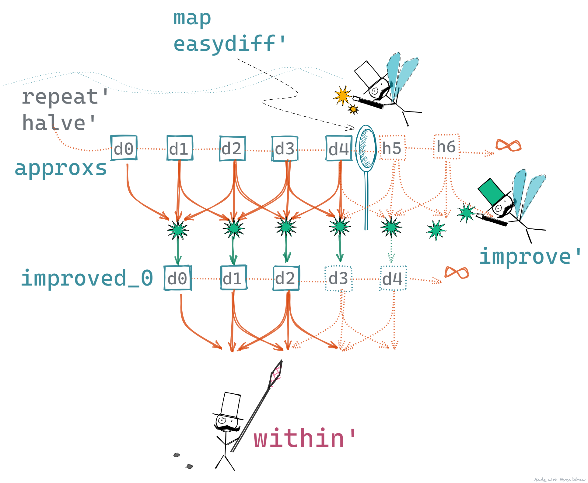
The below picture gives you an idea of how this program works.

• The Selector, keeps demanding for the next value
• On each demand, repeat' halve' produces a value - 1, 0.5, 0.25, 0.125, and so on
• The next value is transformed by the map easydiff' function before within' can read it
• The program stops when within' is satisfied.

Version 2: Improved Differentiation using Numerical Methods ⭐⭐

Now it seems that every approximation can be written as the below

approximation = right answer + error term involving h

We can write the relation between successive approximations as follows.

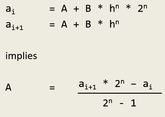
From the above, we can derive the below function to eliminate elimerror' errors using successive approximations. However, elimerror' needs an input n. It turns out that n can be obtained based on three subsequent approximations. Look at order' below.

elimerror' n (a1:a2:rest) = 
  acc : elimerror' n (a2:rest)
  where
    acc = ((a2*(2**n) - a1) / (2**n - 1))
order' a1:a2:a3:rest =
  round $ logBase 2 ((a1-a3)/(a2-a3) - 1)

Note: If it is too much, and I guess it is, you can gloss over the math and just focus on the needs of the functions.

• elimerror' takes in two successive approximations, and returns a much better approximation
• order' takes in three successive approximations, and returns the value for the term n which is fed to elimerror'

We can now define a function improve' that is composed of the above functions. This function is now ready to take in the list of approximations and produce another list of approximations, which will be an improved list of approximations because we eliminate errors as we go. This should make our program terminate faster.

improve' s = elimerror' (order' s) s

Now we can make improved guesses using the below

within' eps $ improve' $ differentiate' sin 2 1

Note: I have introduced the $ operator here. It is used simply to eliminate parentheses. So,

within' eps $ improve' $ differentiate' sin 2 1

simply means

within' eps (improve' (differentiate' sin 2 1))

The below picture gives you an idea of how this changes our program

• The Selector, keeps demanding for the next value - no change here
• On each demand, repeat' halve' produces a value - 1, 0.5, 0.25, 0.125, and so on - no change here
• The next value is transformed by the map easydiff' function - no change here
• Before the value reaches within', we improve upon it
• The improve' method generates another series of values based on the original approximations. These are read by within'
• The program stops when within' is satisfied. - no change here

Hopefully, it would make our Selector walk a little less and make him less tired. And we did this by introducing another infinite sequence.

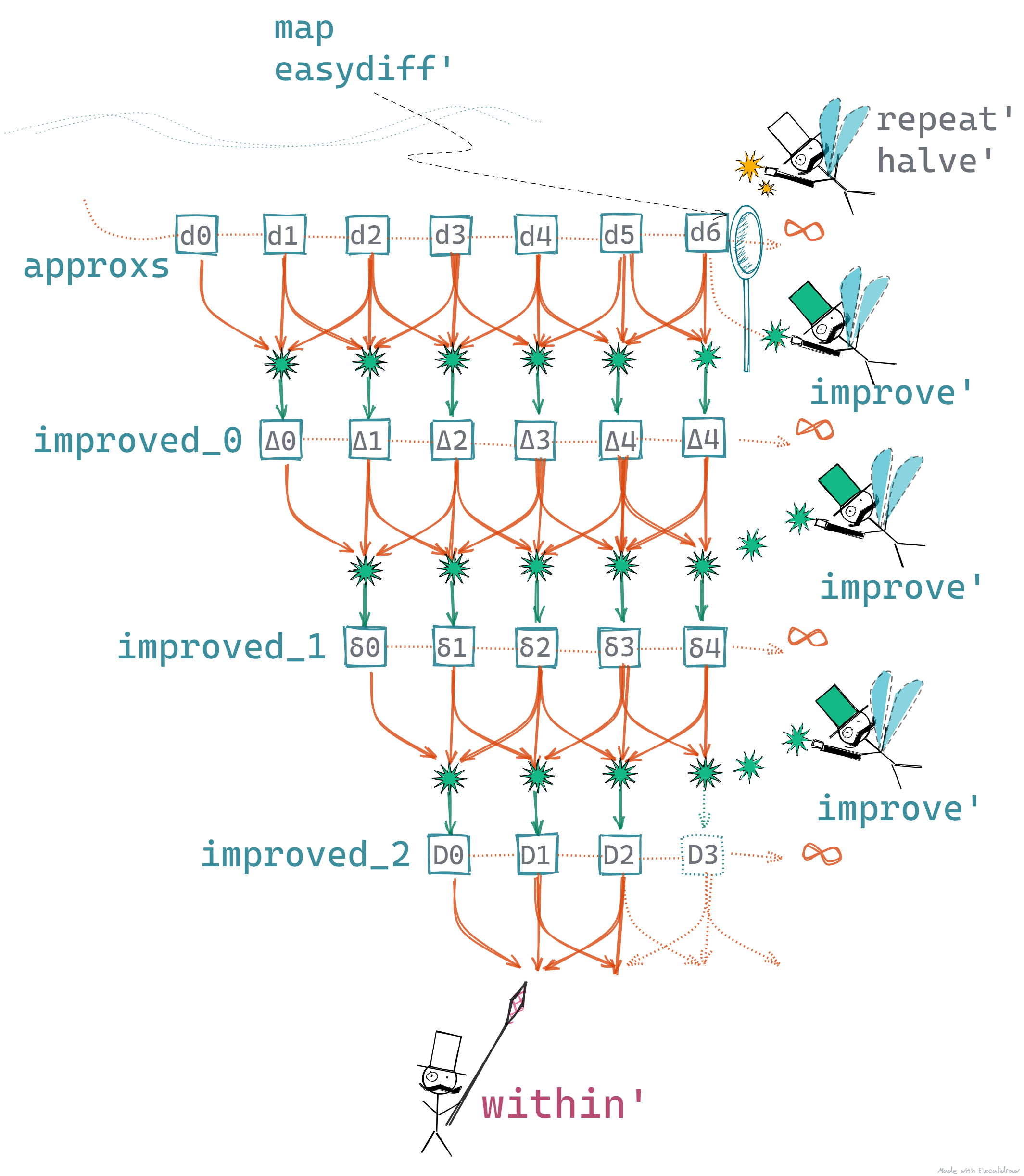
Much Improved Differentiation using Numerical Methods ⭐⭐⭐

Now there is never too much of a good thing, so why just improve the approximations once, why not twice or thrice?

within' eps $
  improve' $
    improve' $
      improve' $
        differentiate' h0 f x

So our original list gets improved upon not once, twice, but thrice. This produces four infinite sequences that are lazily generated and the fourth one i.e. the most improved one is the one that is consumed by the Selector.

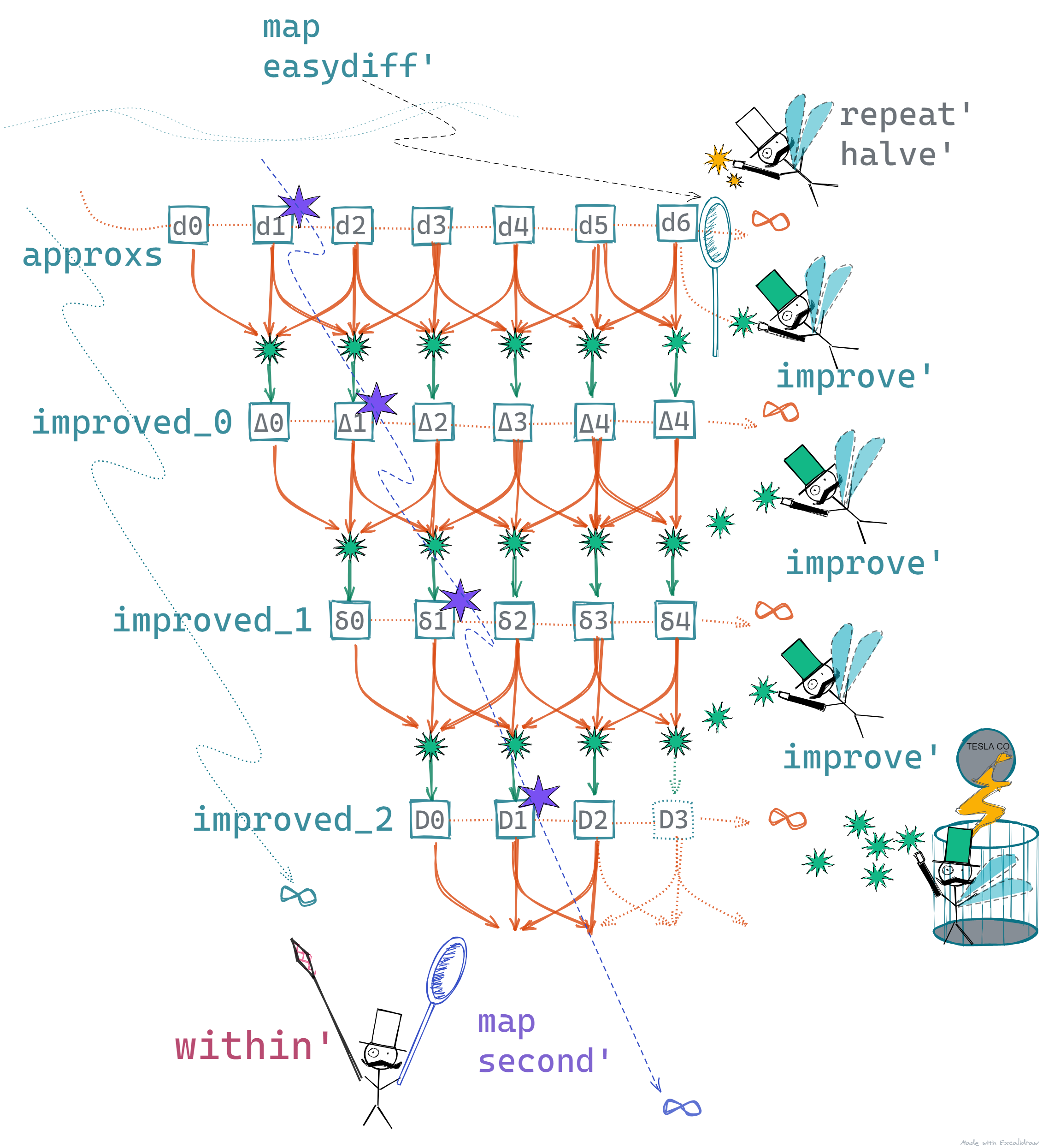
Infinitely Improved Differentiation using Numerical Methods ⭐⭐⭐✨

I know you are greedy for more laziness, so I know that you won't stop at three. Why not try infinitely improving the original approximations? How do we do it? Simple we repeat'!

second' a1:a2:rest = a2
super' s =
  map second' (repeat' improve' s)
within' eps $
  super' $
    differentiate' h0 f x

• We use our function repeat' to create an infinite list of improve' functions
• These get applied to the list of initial approximations one by one to produce intermediate improved lists
• Then output sequences get improved one after the other infinitely! ... but lazily of course 🙂
• Next, we equip our selector with map second' that plucks the second value from each of the lists
• Finally, we use within to terminate the program - no change here

Disclaimer: No magicians were harmed during this implementation.

🎄 Numerical Integration

Picture by Jené Stephaniuk

Integration for a function f between points a and b is the area under the curve between the two points. Similar to differentiation, we can estimate the area under the curve by trying to fit shapes for which we know how to exactly calculate the area. In our case, we can choose the known shapes to be rectangles. The smaller the rectangles, the better they fit under the curve, hence reducing the error value.

Animation by Gregory Leal

Analogous to differentiation, we can start with the below function that takes two points and sums the area of two rectangles

• First one has a height of (f a) and width of (b-a) / 2
• Second one has a height of (f b) and width of (b-a) / 2

easyintegrate' f a b = ((f a) + (f b))*(b-a) / 2

Using the above, we can define a recursive method to create a series of approximations for integration.

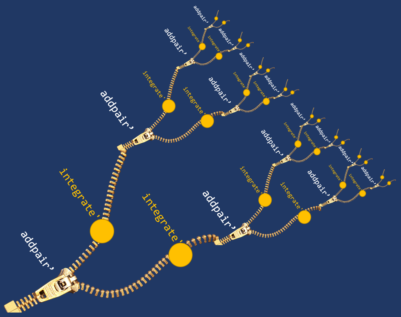
addpair' (a b) = a + b
zip' (a:as) (b:bs) = (a b) : (zip' as bs)
integrate' f a b = (easyintegrate' f a b) : 
                   (map addpair (zip' (integrate' f a mid)
                                      (integrate' f mid b)))
   where mid = (a + b) / 2

• The first value is simply the value of easyintegrate' for f between a and b
• This is followed by a sequence of pairs zipped together each pair is a recursive call to integrate'
• The pairs are combined using the addpair' method, which simply sums them up
• The recursive calls lead to the below where the subsequent calls get further broken down into solving for smaller parts
• These will be eventually aggregated to produce a more accurate result for integration of the f between a and b

The yellow dots are smaller chunks that get put together as the zipper closes in.

We can now call our integrate' method with improve' and within' as below.

within' eps $ super' $ integrate' f 1 2
  where f x = 1/(1 + x*x)

This version of integrate' is a bit inefficient because it re-calculates the values of f for the edges and at the midpoint - (f a), (f b), (f mid), at each stage then recursively on each call to integrate'.

We can modify it a bit to make it more efficient.

integrate'' f a b = integ' f a b (f a) (f b)
integ' f a b fa fb = ((fa+fb) * (b-a) / 2) : 
                     (map addpair' (zip' (integrate'' f a m fa fm)
                                        (integrate'' f m b fm fb)))
   where mid = (a + b) / 2
         fm  = f mid

📝 Conclusion

Phew! That was a lot of math and some pretty complicated calculations but all done using small and simple modules - within', relative', and improve'. We used lazy evaluation to break up the complexity and stick together the smaller pieces.

Summary

1. We continued with lazy evaluation and looked at programs that deal with infinite sequences
2. Out programs were simple and modular
3. With the use of selectors and generators, we wrote programs for Numerical Differentiation and Numerical Integration
4. We further improved our programs by deriving infinite sequences from our initial sequence of approximations
5. We continued to derive infinite sequences and our program didn't blow up, because it ran with strict synchronization and proper terminating conditions

Yet again, we saw how using functional programming helps us write re-usable components and how we can do a lot more with a lot less code. Next in this series, we will get into the final part of the white paper¹. We will see what it takes to make a program that can play a small game.

If you are interested in dabbling around with Haskell, you have the below options.

• You can download and install the Haskell toolchain from here: https://www.haskell.org/downloads/
• OR you can just try it in your browser here: https://www.tryhaskell.org/
• OR ELSE you can just https://repl.it 🙂

If you don't want to get your hands dirty, that's fine too. We'll continue here with the next one in this series - Why FP Matters.

Up Next

Why FP Matters - Part 4 🤖: Let's play!

For more fun stuff like this, click here to see a list of all my posts

Picture by Phillip Glickman